1. Introduction

1.1.1 Introduction

Optimisation shell Inverse is designed for solving inverse and optimisation problems. Simulation programme, typically a finite element method (FEM) based programme is used for evaluation of the objective and constraint functions.

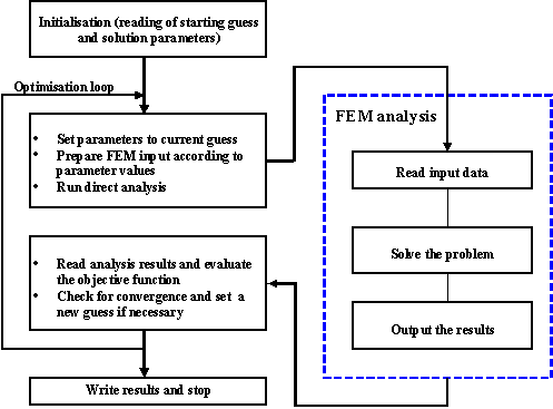
The solution scheme of typical problem solved by the shell is shown in Figure 1. Tasks on the left side of the figure are a part of the optimisation algorithm which minimises the objective function. The right part of the scheme is referred to as “direct analysis” or “simulation”. It represents the main part of the evaluation of the objective and constraint functions and is usually performed by a separate programme or a separate module.

In the solution scheme of optimisation or inverse problems, the shell provides optimisation algorithms and an environment in which one can link these algorithms with the simulation programme which is used for evaluation of the objective and constraint functions and possibly their gradients. Beside optimisation algorithms the shell also provides the user with other tools necessary to approach optimisation problems effectively, i.e. tabulating utilities, some basic mathematical tools, etc. Beside the tools which are directly set for solving optimisation problems, the shell provides tools for manipulating the simulation environment which plays crucial role at the problem definition. At the end, the shell provides an environment in which the user can use both set of tools in order to properly define and solve various kinds of the optimisation problems.

Figure 1: A solution scheme for an optimisation problem.

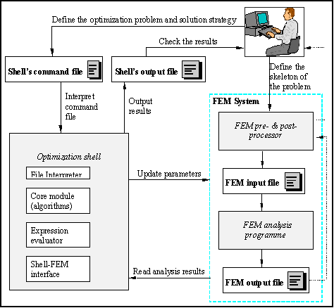
Figure 2 shows how the shell is used in combination with a simulation programme to form a flexible optimisation system for solving inverse and optimisation problems. User of the system defines a skeleton of the direct problems that are successively solved during the optimisation process, by the simulation unit’s pre-processor.

The optimisation problem and the solution strategy are defined through the shell’s command file. To ensure high flexibility at defining various problems, the command file syntax resembles a high level programming language. All necessary supporting utilities like optimisation algorithms, function definition facilities, mathematical tools (function approximation, matrix operations, etc.) and interfacing with the direct simulation, are provided through the pre-defined shell interpreter’s functions. Data transfer between these utilities, implemented as separated modules of the shell, is provided through the shell’s global variables.

In the solution procedure the shell interprets the command file. Everything what happens is either explicitly or implicitly defined in the command file. Typically, the core part of the solution procedure is a built-in optimisation algorithm, whose execution is triggered from the command file. The algorithm successively executes direct problems at different sets of the design parameters. Direct problems are defined in a special block of commands in the command file. The simulation interfacing functions are used to properly update the direct analysis definition according to the design parameters and to read and combine the analysis results to form the information needed by the optimisation algorithm (i.e. the objective and constraint functions values and their derivatives with respect to the design parameters).

Figure 2: Scheme of the optimisation system which consists of the shell and an optimisation programme.

2.1.1 File Interpreter

User of the optimisation system accesses all built-in tools of the optimisation shell through the file interpreter’s functions. When the shell is run, its file interpreter interprets the command file written by the user and executes the appropriate actions.

Syntax of the command file is very simple. It consists of function names each of which is followed by an argument block in curly brackets. Curly brackets following function names are necessary even when functions take no arguments (in this case brackets are empty).

The order in which functions should be called is not defined in advance and is affected only by the logics of the procedure which is defined through the command file. For example, if we run commands which operate on files, we must take care about opening the appropriate files first. If we run an optimisation algorithm, we must previously define how the objective and constraint functions, etc., are evaluated.

The file interpreter does not enforce any rules how arguments should be passed to functions through the argument list. It is the matter of the interpreter’s functions how they interpret arguments in their argument blocks. Some general rules are set about format of specific types of arguments, however functions can be written which don’t obey these rules completely. These functions are exceptional and in the instructions for their use the formats of their argument lists are is always exactly described.

Beside functions which trigger pre-defined algorithms and built-in tools of the shell, there are also flow control functions, i.e. functions which enable branches and loops. The rules for these functions are the same as for the others. It is typical for them that their argument lists contain blocks of commands which are interpreted by the interpreter if certain conditions are fulfilled. These conditions are specified by the user in the form of mathematical expressions which are evaluated by the shell’s expression evaluator. Expression evaluator is a special module of the shell which enables evaluation of mathematical expressions.

Here is a simple example of the use of the while loop:

={i:1}

while{ (i<=10)

[

={i : i+1}

write{“ i = “ $i \n}

]}

The first function (=) sets expression evaluator’s variable i to 1. This variable is also created because it has not existed before. The while function which is an implementation of the while loop follows. The function takes two arguments: the first one is condition – a mathematical expression in round brackets. The second one is a block in square brackets which is successively executed (interpreted) while the condition is fulfilled, i.i. while the expression in round bracket evaluates to a non-zero value. In the present example, we add 1 to variable i and write its value while it is not greater than 10.

Beside the while loop, the interpreter knows the do loop and the if/else branch. syntax is the following:

while { (expression) [block] }

do { [block] (expression) }

if { (expression) [block1] < else [block2] > }

The do function executes the block in square brackets until the value of the expression in the round brackets becomes zero. The if function executes the block in the first square brackets if the expression in the round brackets evaluates to zero. Otherwise it executes the block in the second square brackets in the case it is given (this block is optional, which is indicated by angle brackets in the if command syntax definition). The word else is meaningless for the interpreter, but can be added for clearness of the code.

The user can define new interpreter functions by the interpreter. This can be done bz the interpreter-s function function with the following syntax:

function {name (arguments) [definition] }

name is the name of new interpreter-s function defined this way. arguments is the round brackets is a list of formal arguments where their names are separated by spaces. The definition block follows in the square brackets. Every time the newly defined function is called in the command file, all appearences of formal parameters in the definition block are replaced by real parameters on the string bases and then the defiition block is intepreted. The appearences of formal parameters in the definition block are designated by argument names preceeded by the “#” sign.

2.1.2 Expression evaluator (calculator)

Expression evaluator (also referred to as calculator) serves for evaluation of mathematical expressions given as string arguments of the file interpreter's functions. Its important use is in flow control functions for evaluation of conditions for loops and branches. Normally, mathematical expressions can also be used in place of numerical arguments of the file interpreter’s functions (there are some rare exceptions).

There are two interpreter’s functions which manipulate the expression evaluator’s system, i.e. = and $. The = function assigns a numerical value to a calculator’s variable and creates that variable if it has not been defined yet. The $ function assigns a definition to a calculator’s variable or function. This function also creates an object anew if it has not been defined yet.

Here is an example how these functions can be used:

= { b : 3*4 }

$ { c : b+2*a }

= { a : b/3 }

$ { f1[x,y] : a*f2[x] }

$ { f2[t] : t*t }

= { b : f2[a] }

With the first = function we assign the value of expression “3*4”, i.e. 12, to the expression evaluator’s variable b which is also created since it has not existed before. With the $ command which follows we define a new variable c so that it represents the expression “b+2*a”. This expression does not have a defined value since the variable a has not been defined yet. The definition of b is symbolical and its value will not be defined until we define a. This is done with the next = function which creates the variable a and assigns the value of the expression “b/3”, i.e. 4, to it. With the next $ function we define a new calculator’s function named f1. It is defined the expression “a*f2[x]” where a refers to a expression evaluator’s variable, x and y will be at function evaluation replaced by the arguments with which function is called, and f2 is the expression evaluator’s function named f2 which is at this point not defined. The definition is again symbolical, so it will be able to use the newly defined function in expression evaluations as soon as the function f2 is defined. This is done in the next line where we define function f2 as square of its only argument. In the last line we assign the value of expression “f2[a]” to variable b. The value of b so becomes 16 instead of 12, since the value of a is 4 and the function f2 evaluates to square of its only argument by the definition made in previous line. Because the value of b has been changed, the value of c in expressions also changes because c is defined through an expression which contains the variable b. The value of a does not change, because the present value of the expression “b/3” has been assigned to a, not the expression itself.

The expression evaluator has pre-installed some basic mathematical functions like trigonometric and hyperbolic functions, and it knows basic algebraic operators like +, *, -, etc. The user can arbitrarily combine these functions and operators to define new evaluator’s variables and functions. Besides, new functions can also be defined through the shell’s file interpreter by the function definefunction. At each evaluation of such function its definition block is interpreted.

Of special importance are the pre-defined expression evaluator’s functions through which the user can access the global variables of the shell. All relevant data are stored in such variables during the shell’s execution. Through the appropriate expression evaluator’s functions these data can be used in the flow control conditions or as arguments to file interpreter’s functions. This way, results of shell’s algorithms can be used as input for another algorithms and unlimited data transfer between different modules and utilities of the shell is provided.

2.1.3 User defined variables

User defined variables are used for data storage and data exchange between modules and utilities of the shell. Different types of variables (i.e. scalar, vector, matrix or field variables) enable storage of different types of data. These variables are separated from the expression evaluator, but for most of their types there are pre-defined evaluator’s functions which can access numerical data stored in them. Each variable type has its own set of interpreter’s and evaluator’s functions for handling variables of that type. This includes creating, copying and renaming variables and setting and accessing data stored in them.

Each user-defined variable can contain a multi-dimensional table of elements of a certain type. This enables grouping of pieces of data with similar meaning. Number of dimensions of such element table will be referred to as variable rank. Number of elements which a variable can hold equals products of its dimensions, or 1 if the variable rank is 0. Rank and dimensions of variables are specified by user when they are created by appropriate functions.

In argument blocks of file interpreter’s functions specific data element are referred by variable element specifications. These consist of a variable name and an optional index specification. Index specification is a list of indices in square brackets which specify the position of data element in the variable’s element table. It must be given if the rank of the appropriate variable is different than zero. Let’s say that the user has defined a vector variable named “v1” which holds a three-dimensional table of vectors with dimensions 2, 4 and 3. The last of its 34 elements is then referred to as “v1[2,4,3]” or “v1[2 4 3]”.

Some variables have a pre-defined meaning and are reserved for carrying exactly specified information. For example, a scalar variable named objectivemom holds the lastly evaluated objective function(s) during the execution of optimisation algorithms. Pre-defined variables serve for automatic storage of important intermediate or final results of algorithms and for transfer of data between direct analyses and optimisation algorithms.

2.1.4 Connection with the Simulation Programme

Optimisation algorithms consequently evaluate the objective and constraint functions (and possibly their derivatives), which are defined via the simulation. The optimisation shell must therefore provide a mechanism of defining how the constraint and objective functions are evaluated, take care for performing this evaluation in the optimisation algorithms and enable proper data transfer between optimisation algorithms and direct analysis.

Two concepts are crucial for providing this functionality. First, the evaluation of the objective and constraint function is performed via interpretation of a specific block of code in the command file in which the user exactly defines how these functions are evaluated, together with execution of the simulation programme and necessary interfacing with simulation input and results. By convention this is the argument block of the interpreter’s function analysis.

Second, transfer of data between the shell’s built-in algorithms or utilities and the direct analysis defined by the user through the argument block of the analysis function is implemented through the shell’s variables with pre-defined meaning. When an optimisation algorithm requires evaluation of the objective and constraint functions, the parameters at which the direct analysis should be performed are written to the vector variable parammom and then the argument block of the analysis function is interpreted. Within this block, which defines the direct analysis, parameter values can be accessed through vector variable parammom and used in interface functions to update the simulation input according to these parameter values. The file interpreter’s and expression evaluator’s functions are then used to run the simulation, collect its results relevant to the optimisation algorithm and to evaluate the necessary functions like the objective and constraint functions and their gradients. At the end of the analysis function argument block the evaluated data must be stored in the appropriate pre-defined variables where the optimisation algorithm can pick them. For example, the objective function values must be stored in the scalar variable objectivemom.

In fact there is another interface function between each optimisation algorithm and the direct analysis definition. This function is called in the algorithm’s code when the evaluation of the objective or constraint function is required. It stores its input argument (vector of parameters set by the optimisation algorithm) to the scalar variable parammom, interprets the argument block of function analysis, and returns data stored in the appropriate global variables to the optimisation algorithm.

2.2 Running Direct Analysis

The simplest use of the shell is for parametric studies, i.e. for running direct analyses at different sets of parameters. Even when an inverse or optimisation problem needs to be solved it is recommended that direct analysis is run first to test if the problem was set correctly and there are no problems with the simulation.

In this chapter an example of how to prepare a command file for running a direct analysis at a specific set of parameters is shown. The file is prepared for inverse analysis with two parameters and four measurements. The meaning of specific commands is explained and some conceptual details are discussed on the example.

2.3 An Example of Running Inverse Analysis

An example code of how to run an inverse analysis is shown in this chapter. The parts of the command file are explained and some conceptual details are discussed.

2.3.1 Problem description

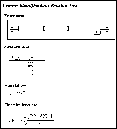
The example deals with inverse identification of hardening parameters of the potential law for the hardening curve. The identification is performed on the basis of experimental data obtained with the tension test where forces at different elongations of the specimen are measured (Figure 3). Model parameters C and n are obtained by minimising the function

, (1)

where are measured forces at different elongations; are the respective quantities calculated with the finite element model by assuming trial values of parameters C and n; are the expected errors of the appropriate measurements and is the number of measurements.

Figure 3: Inverse identification of hardening parameters from results of the tension test.

2.3.2 Command file for the optimisation shell

The code in the shell’s command file which solves the problem is given below. Line numbers are added because of easier referencing. Functions comment or * are used for comments. These functions do nothing, so what is in their argument blocks can be used for in-code comments.

1. comment { beginning of the command file }

2. setfile{outfile “test.ct”} *{output file of the shell}

3. setvector{ meas 4 {1:62200} {2:67800} {3:68900} {4:68000} } *{ vector of measurements}

4. setvector{ sigma {1 1 1 1} } *{ vector of measurement erors }

5. *{ Definition of a new function in expression evaluator: }

6. ${force[inc]: nodreac[inc,4,1] +nodreac[inc,5,1] +nodreac[inc,6,1] +nodreac[inc,7,1] +nodreac[inc,8,1] }

7. analysis

8. {

9. *{ beginning of the “analysis” block }

10. setfile{aninfile “test.dat”} *{ simulation programme’s input file }

11. initinput{} *{ initialization of interface }

12. setparam{} *{ updating parameters in simulation programme’s input data }

13. system{“elfen16 test”} *{ running a simulation programme }

14. setfile{anoutfile “test.res”} *{ simulation programme’s output file }

15. initoutput{} *{ initialization of interface }

16. meas{1 “force[1]”} *{ setting components of simulated measuremets }

17. meas{2 “force[2]”}

18. meas{3 “force[3]”}

19. meas{4 “force[4]”}

20. * { end of the analysis block }

21. }

22. setoption {autochi2}

23.

24. setvector{ parammom 2 {1276 0.1124} } *{ setting vector of parameters }

25. analyse{} *{ running analysis at given prameters }

26.

27. setvector{parammom 2}

28. inverse *{ running inverse analysis }

29. {

30. nd simplex 0.001 300

31. 3 2

32. {

33. {1 1: 1000 }

34. {1 2: 0.1 }

35. {2 1: 1100 }

36. {2 3: 0.1 }

37. {3 1: 1000 }

38. {3 2: 0.11 }

39. }

40. }

41. comment{ end of the command file }

With the setfile command in the second line the file outfile is open. The first argument of the command is the internal name of the file and the second argument is the name of physical file on the disk which is connected with this name. outfile is by convention a file into which results of shell’s operations are written, so from this point on the output of shell’s functions will be written to the file named test.ct. Functions also print their output to the standard output of the shell (usually the terminal window in which the shell was run). The setfile function can also take the third argument which specifies how the file is open. In this case the file is open only for writing which is a convention for the pre-defined file outfile. If the file exists before it is overwritten.

The setvector command in line 3 creates the vector variable meas and sets its only vector element as specified in its argument block. Vector dimension (4) is specified first, then the component values follow. meas is a vector variable with pre-defined meaning and holds the measurements for inverse analysis.

With the next setvector command vector sigma (vector of measurement errors) is set. sigma is also a vector variable with a pre-defined meaning which have by definition the same dimension as the vector meas. Since this dimension is already known because it was specified when vector meas was set, it does not need to be specified again and therefore only the four vector components are set. Vectors can be given in various different formats which will be discussed later.

A new expression evaluator’s function force is defined by the $ command in line 6. This function will return the simulated forces at increments specified by the only arguments. These forces will be extracted from the simulation output by the expression evaluator’s built-in functions nodreac. These functions are a part of the shell-simulation interface and can extract nodal reactions from the output of the finite element simulation programme. This function is at the moment available only for the FEM programme Elfen and extract data only for programme’s output file. The shell-simulation interface must be initialised before this function is evaluated. For some other simulation programmes interfaces will be available in the future. When the interface with a particular simulation programme is not implemented in the shell, the general file interface utilities can be used to extract the data from the simulation output file. With this utilities data can be obtained from any text output file with a known format, but this requires few additional lines in the command file. The user can also build the whole set of interfacing functions based on the general file interface utilities.

With the analysis command in line 7 it is specified how the direct analysis at specific parameter values is performed. The argument block of this commmand is interpreted by the shell’s file interpreter every time the direct analysis is performed. Therefore interpretation of this block is a part of evaluation of the objective and constraint functions and possibly their derivatives with respect to parameters. Execution of the analysis function itself does not do much, actually it only stores the position of its argument block so that it can be found and interpreted when the evaluation of the objective or constraint functions or their gradients is requested.

The first command in the argument block of the analysis command, setfile in line 10, connects the file variable aninfile with the file test.dat and opens that file. The file is open for writing since aninfile ia a pre-defined file variable used for the simulation input file. The next command, initinput, initialises the shell’s interface with the simulation programme’s input file. This command must be executed before using functions for setting input data for the simulation. This is the property of current interface with the finite element programme Elfen and is not in general valid for interfacing with other simulation programme (see references for interfaces with other programmes or the reference for the general file interface) Among the others, the initinput command sets the file on which the interface functions will operate to the file connected with the file variable aninfile.

The setparam function which is called next is a part of the file interface. This function sets the current values of input parameters in the simulation’s input file. These values are found in the vector variable parammmom, which by convention holds current parameter values. In the interface with Elfen, the user must designate the placer in Elfen’s input file where the parameters must be updated, so that the setparam function can find these places and update the appropriate values. Again, different rules apply to other interfaces.

The system command in line 13 runs the simulation programme with the updated input data which is in this case read from file. At the rest of the analysis function’s argument block, the necessary results are read and the appropriate function values (like the objective function) are evaluated.

The setfile function in line 14 sets connects the file variable anoutfile with the file test.res and opens that file for reading. anoutfile is also a pre-defined file variable which represents the analysis output file.

The initoutput command initialises the part of the interface which interact with the analysis output. It must be executed before the interface functions for extracting results are called or evaluated.

The next four calls of the meas function (lines 16 to 19) specify how the values of the vector measmom will be calculated. The first argument of each function is the number of component which is evaluated and the second argument is a mathematical expression in double quote, the value of which is assigned to that component. The function meas evaluates the expression by the expression evaluator and assigns its value to the appropriate component of vector measmom. In all four cases, expressions include the expression evaluator’s function force which was defined in line 6. This function includes calls to the expression evaluator’s function nodreac which is a part of the shell’s interface with the simulation programme Elfen. This function evlauates to a specific component of the nodal reaction at a specific node after a specific increment. The increment number, node number and component are arguments of the function, while the returned information is extracted from the simulation output file which becomes known to the interface when the initoutput command is executed.

The value of the objective function is in this case calculated automatically in this case from measurements meas, measurement errors sigma and simulated measurements measmom according to formula (1). This value is written to the scalar variable objectivemom after the analysis function’s argument block is interpreted. Automatic evaluation of the objective function is instructed by setting the autochi2 option which can be used at inverse analyses. When optimisation is in question, we must always explicitly specify at the end of the analysis command’s argument block how the objection function is calculated.

In lines 24 and 25 a direct analysis is run at specific values of parameters. First we set the current vector of parameters parammom and then run the direct analysis by the analyse command. This command triggers the interpretation of the analysis function’s argument block and the prints the results of the analysis, i.e. prints the pre-defined variables in which results are stored by convention.

The inverse command in line 28 executes the inverse analysis, i.e. the algorithm which minimises the objective function. The first two parameters specify the algorithm which is used (the simplex method in this case), then a tolerance for function minimum and maximum allowed number of iteration are given and the last argument is a matrix of initial guesses. This matrix is given in a standard format in which matrices are specified in the shell. The simplex method requires one more initial guesses than the number of parameters. A setvector function is called before the call to inverse, but only the dimension of vector parammom was specified, not the components. These are set subsequently by the optimisation algorithm when it runs direct analyses.

Whenever the optimisation algorithm wants to evaluate the objective or constraint functions or their derivatives, it calls the appropriate shell’s internal function for direct analysis. This function first copies the parameters, which are its input arguments set by the optimisation algorithms, to the vector variable parammom, and then triggers interpretation of the argument block of the analysis command. At the end it passes the appropriate pre-defined variables to the optimisation algorithm, according to what it has requested. In the analysis function’s argument block the user defines the way how different functions requested by the optimisation algorithm are calculated at a specific set of parameters. The parameter values set by the algorithm can be accessed through the pre-defined vector variable parammom. The user must programme the way how the simulation input data is updated according to parameter values, how the simulation is performed and how the needed data is evaluated and written to the appropriate pre-defined variables. The shell’s internal function for the direct analysis then passes the appropriate results to the optimisation algorithm.